---
title: "Package Documentation"
format:
html:
toc: true
code-fold: true
code-tools: true
execute:
echo: true
warning: false
message: false
---
## Overview
This project is organized into two main components:
1. **Data acquisition and construction (`fetch_data.py`)**
Pulls raw Statcast data, aggregates hitter-level summaries, merges in barrel metrics, and saves a cleaned CSV used throughout the project.
2. **Analysis utilities (`analysis.py`)**
Loads the combined dataset, applies consistent filtering, and provides functions for generating tables, correlations, outlier summaries, and plots used in both the report and Streamlit app.
Generally you will not need to run `fetch_data.py` directly and can instead work from the saved dataset using the analysis functions.
## Data Acquisition and Dataset Construction (`fetch_data.py`)
This project includes a standalone script, `fetch_data.py`, which constructs the season-level hitter dataset used by the analysis module and Streamlit app. The script collects Statcast event-level data for the 2025 season, filters to home runs, aggregates hitter-level summaries, and merges in barrel statistics from a separate Baseball Savant leaderboard export. The final output is a single combined CSV used throughout the project.
### What the script produces
Running `fetch_data.py` creates the following files:
- `data/hr_distance_leaders_2025.csv`
Player-level home run summaries computed directly from Statcast event data (home run count, average/max distance, average/max exit velocity).
- `data/combined_leaders_2025.csv`
The final analysis dataset containing the home run summaries merged with barrel metrics (barrels and barrel percentage).
### Data sources
The dataset is assembled from two sources:
1. **Event-level Statcast data via `pybaseball`**
The script uses `pybaseball.statcast()` to collect pitch-by-pitch data for the 2025 season and filters to `events == "home_run"`. This provides the raw inputs for home run distance and exit velocity metrics.
2. **Barrel leaderboard data from Baseball Savant**
Barrel totals and barrel percentage are imported from `data/exit_velocity.csv`, which is a leaderboard-style CSV downloaded from Baseball Savant.
### Processing steps
The script follows these steps:
1. **Pull Statcast data for the full season**
- `statcast(start_dt="2025-03-20", end_dt="2025-11-01")`
2. **Filter to home runs only**
- `hr = data[data["events"] == "home_run"]`
3. **Aggregate to hitter-season level**
Grouping by hitter ID (`batter`), the script computes:
- `hr_count`: number of home runs
- `avg_hr_distance`, `max_hr_distance`: mean and max of `hit_distance_sc`
- `avg_launch_speed`, `max_launch_speed`: mean and max of `launch_speed`
4. **Apply minimum sample size threshold**
- Only hitters with `hr_count >= 5` are kept.
5. **Round numeric columns for readability**
- Distance and exit velocity are rounded to 1 decimal place.
6. **Load and clean barrel leaderboard data**
- The leaderboard file `exit_velocity.csv` is loaded.
- A `player_name` field is created from the `"last_name, first_name"` column.
- Only `player_id`, `player_name`, `barrels`, and `brl_percent` are retained.
7. **Merge datasets**
- The home run summary table is merged with the barrel table using IDs:
- `leaders.batter` matched to `savant_barrels.player_id`
- The merge uses `how="inner"` to keep only hitters present in both sources.
8. **Finalize columns and save**
- Columns are ordered so that `player_name` appears first.
- The final dataset is saved to `data/combined_leaders_2025.csv`.
### How to run it
From the repository root:
```bash
python fetch_data.py
```
## Analysis Module (`analysis.py`)
The `analysis.py` module contains the core analysis functionality used throughout this project. It is designed to operate on the cleaned, season-level Statcast dataset produced by `fetch_data.py` and saved as `combined_leaders_2025.csv`.
The functions in this module support:
- loading the combined dataset
- applying consistent filtering rules
- generating summary and ranking tables
- computing correlations among power metrics
- identifying outliers using z-scores
- producing scatter plots used in both the report and Streamlit app
All analysis is performed at the **player-season level**, meaning each row represents a hitter summarized across the season.
---
## Design
The analysis module is intentionally lightweight and modular. Each function:
- performs a single, well-defined task,
- does not modify inputs in place,
- returns either a pandas DataFrame or a Matplotlib figure,
- can be reused in scripts, reports, or interactive applications.
This design allows the same code to power the static report and the interactive Streamlit app without duplication.
---
## Loading and Preparing Data
#### `load_combined(path=COMBINED_CSV)`
Loads the combined hitter dataset from disk.
**Purpose**
- Provide a single entry point for loading the cleaned Statcast leaderboard dataset.
**Parameters**
- `path` (`Path | str`, optional): Path to the combined CSV file. Defaults to `data/combined_leaders_2025.csv`.
**Returns**
- `pd.DataFrame`: DataFrame containing hitter-level statistics.
**Example**
```{python}
from stat386_project.analysis import load_combined

df_raw = load_combined()
df_raw.head()
```
---
### `prepare_data(df, min_hr=5, dropna_cols=None)`
Filters and cleans the dataset used for analysis.
**Purpose**
- Remove hitters with very small sample sizes.
- Ensure all required metrics are present before analysis.
**Parameters**
- `df` (`pd.DataFrame`): Input DataFrame.
- `min_hr` (`int`, default `5`): Minimum number of home runs required.
- `dropna_cols` (`Iterable[str] | None`): Columns that must not contain missing values.
If `None`, defaults to:
- `avg_hr_distance`, `max_hr_distance`
- `avg_launch_speed`, `max_launch_speed`
- `barrels`, `brl_percent`
**Returns**
- `pd.DataFrame`: Filtered copy of the DataFrame.
**Notes**
- The function returns a copy and does not modify the input DataFrame.
- Most downstream functions assume this filtering step has already been applied.
**Example**
```{python}
from stat386_project.analysis import load_combined, prepare_data

df = prepare_data(load_combined(), min_hr=5)
df.shape
```
---
## Summary and Ranking Tables
### `longest_vs_avg_distance(df, n=20)`
Creates a ranking table of hitters by **maximum home run distance**, with average distance and exit velocity context.
**Purpose**
Compare extreme peak power with typical home run distance.
**Parameters**
- `df` (`pd.DataFrame`): Cleaned dataset.
- `n` (`int`, default `20`): Number of hitters to return.
**Returns**
- `pd.DataFrame`: Top `n` hitters sorted by `max_hr_distance`.
**Example**
```{python}
from stat386_project.analysis import longest_vs_avg_distance

longest_vs_avg_distance(df, n=10)
```
---
### `barrel_power_table(df, n=20)`
Ranks hitters by barrel percentage and reports related power metrics.
**Purpose**
Examine how contact quality aligns with distance and exit velocity metrics.
**Parameters**
- `df` (`pd.DataFrame`): Cleaned dataset.
- `n` (`int`, default `20`): Number of hitters to return.
**Returns**
- `pd.DataFrame`: Top `n` hitters sorted by `brl_percent`.
**Example**
```{python}
from stat386_project.analysis import barrel_power_table

barrel_power_table(df, n=10)
```
---
### `workload_vs_distance(df)`
Returns a table relating home run workload to average distance.
**Purpose**
Explore whether hitters with more home runs tend to hit longer home runs on average.
**Parameters**
- `df` (`pd.DataFrame`): Cleaned dataset.
**Returns**
- `pd.DataFrame` with columns:
- `player_name`
- `hr_count`
- `avg_hr_distance`
**Example**
```{python}
from stat386_project.analysis import workload_vs_distance

workload_vs_distance(df).head()
```
---
## Correlation and Outlier Analysis
### `correlation_table(df)`
Computes a Pearson correlation matrix for key power-related metrics.
**Purpose**
Quantify linear relationships among distance, exit velocity, barrel metrics, and home run totals.
**Included metrics**
- `avg_hr_distance`
- `max_hr_distance`
- `avg_launch_speed`
- `max_launch_speed`
- `barrels`
- `brl_percent`
- `hr_count`
**Parameters**
- `df` (`pd.DataFrame`): Cleaned dataset.
**Returns**
- `pd.DataFrame`: Correlation matrix.
**Example**
```{python}
from stat386_project.analysis import correlation_table

correlation_table(df).round(3)
```
---
### `find_outliers(df, columns=('avg_hr_distance','max_hr_distance','avg_launch_speed'), z_thresh=2.5)`
Identifies hitters with extreme values on selected metrics using z-scores.
**Purpose**
Highlight standout performance profiles rather than treat them as errors.
**Parameters**
- `df` (`pd.DataFrame`): Cleaned dataset.
- `columns` (`Iterable[str]`): Metrics used for z-score computation.
- `z_thresh` (`float`, default `2.5`): Threshold for flagging outliers.
**Returns**
- `pd.DataFrame`: Subset of hitters flagged as outliers.
**Notes**
- Z-scores are computed using population standard deviation (`ddof=0`).
- A hitter is flagged if **any** selected metric exceeds the threshold in absolute value.
**Example**
```{python}
from stat386_project.analysis import find_outliers

outliers = find_outliers(df)
outliers[["player_name", "avg_hr_distance", "avg_hr_distance_z"]].head()
```
---
## Plotting Functions
All plotting functions return Matplotlib figure objects.
---
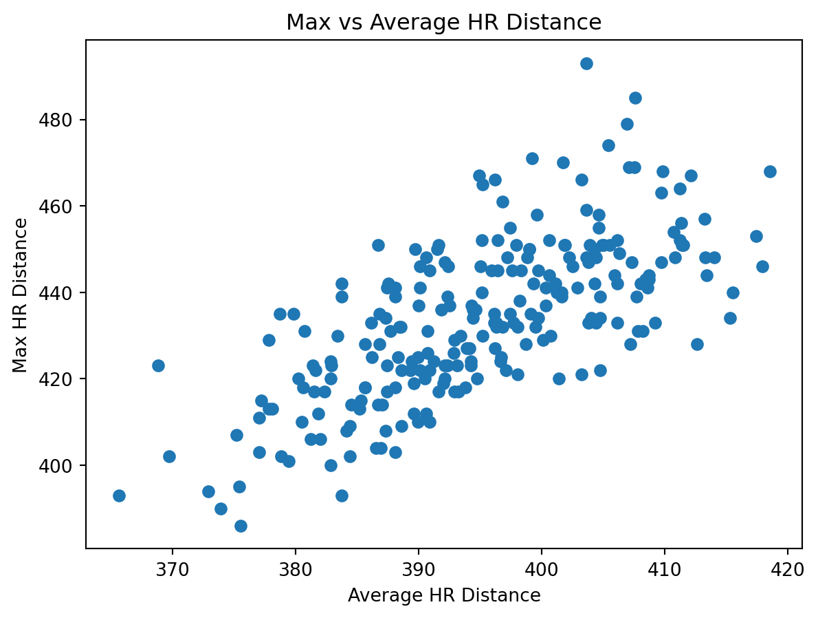
### `plot_max_vs_avg_distance(df)`
Scatter plot of average home run distance versus maximum home run distance.
**Purpose**
Visualize the relationship between peak and typical power.
**Returns**
- Matplotlib graph
**Example**
```{python}
from stat386_project.analysis import plot_max_vs_avg_distance

fig = plot_max_vs_avg_distance(df)
fig
```
---
### `plot_launch_speed_vs_distance(df)`
Scatter plot of average exit velocity versus average home run distance.
**Purpose**
Examine whether harder contact corresponds to longer average home runs.
**Returns**
- Matplotlib graph
---
### `plot_barrel_percent_vs_distance(df)`
Scatter plot of barrel percentage versus average home run distance.
**Purpose**
Explore the relationship between contact quality and average power.
**Returns**
- Matplotlib graph
---
### `plot_hr_count_vs_distance(df)`
Scatter plot of home run count versus average home run distance.
**Purpose**
Examine how workload relates to typical power outcomes.
**Returns**
- Matplotlib graph